Data Preparation and Feature Engineering for Machine Learning: A Practical Guide with pandas and scikit learn Pipelines

Most beginners think machine learning is about choosing the right algorithm. In practice, the model is the easy part. The real work, and the part interviewers love to probe, is getting raw data into a clean, honest shape that a model can learn from. This guide walks you through data preparation and feature engineering step by step using the Titanic dataset, which loads directly through seaborn, so you can follow along in Google Colab or Kaggle without downloading anything.

By the end, you will have one reusable scikit-learn Pipeline that handles missing values, encoding, scaling and modelling together, and you will understand how it protects you from the most common mistake in student projects: data leakage.

Step 1: Explore the Data Before You Touch It

Never start cleaning blindly. Ask three questions: what does each column mean, what type is it, and what is the target?

import seaborn as sns
import pandas as pd

df = sns.load_dataset("titanic")
print(df.shape)
print(df.head())
df.info()
print(df.describe())
print(df["survived"].value_counts(normalize=True))

There are 891 passengers and 15 columns. The target survived is binary, and roughly 38 percent survived, so the classes are somewhat imbalanced. The maximum fare sits far above its 75th percentile, which hints at outliers. Some columns duplicate others: class mirrors pclass, embark_town mirrors embarked, and alive is just survived written as yes or no. Spotting these early prevents serious bugs later.

Key takeaway: df.info(), df.describe() and value_counts() are your first three commands on any new dataset.

Step 2: Clean Missing Values and Outliers

Missing values

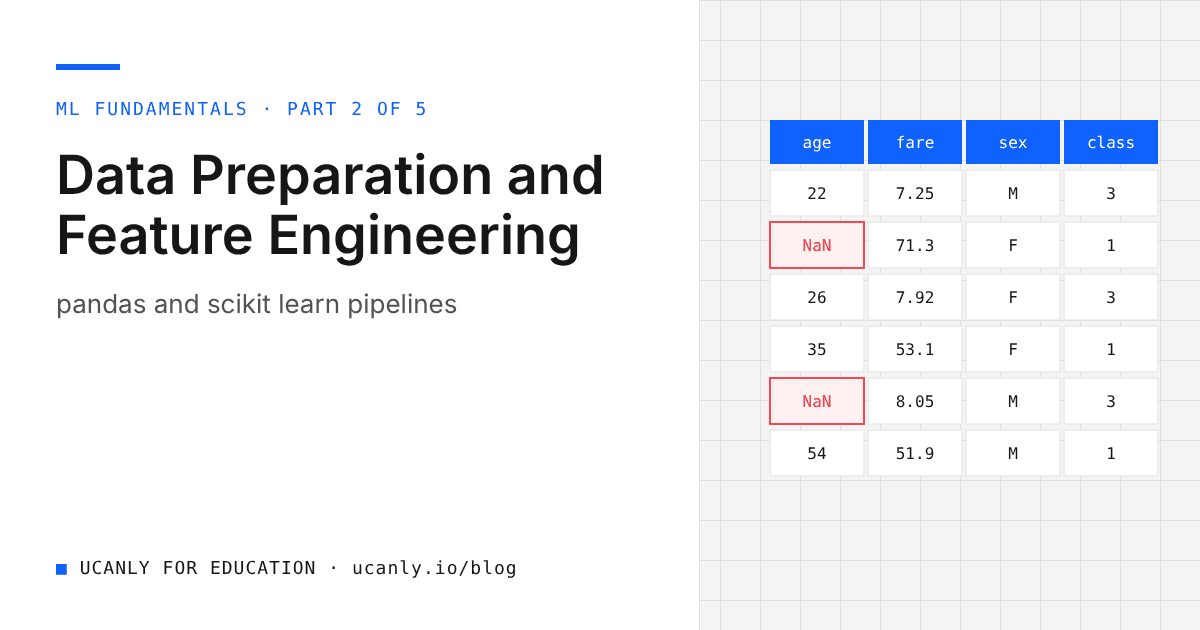
Missing data is normal, whether it is a placement record with blank CGPA fields or an internship form with optional columns. The question is how much is missing and why.

import seaborn as sns
df = sns.load_dataset("titanic")
print(df.isna().sum().sort_values(ascending=False).head(5))
print((df.isna().mean() * 100).round(1).sort_values(ascending=False).head(5))

In this run, deck is missing for about 77 percent of rows, age for about 20 percent, and embarked for just two rows. Each calls for a different decision:

• Mostly empty columns like deck: usually drop them. Filling 77 percent of a column with guesses adds noise, not information.
• Moderately missing numeric columns like age: impute with the median, which is robust to extreme values. The mean gets pulled by outliers.
• A few missing categorical values like embarked: impute with the most frequent category.

The important rule: whatever value you fill in must be computed from the training data only. We will enforce that automatically with SimpleImputer inside a Pipeline.

Outliers

A common detection rule uses the interquartile range (IQR): anything above Q3 plus 1.5 times the IQR is flagged.

import seaborn as sns
df = sns.load_dataset("titanic")
fare = df["fare"]
q1, q3 = fare.quantile([0.25, 0.75])
iqr = q3 - q1
upper = q3 + 1.5 * iqr
print("Upper fence:", round(upper, 2))
print("Rows above fence:", (fare > upper).sum())
print(df.loc[fare > upper, "pclass"].value_counts())

The IQR rule flags over a hundred fares as outliers, and almost all of them belong to first class passengers. That is the lesson: an outlier is not automatically an error. These are genuine expensive tickets, and they carry real signal about survival. Deleting them would throw away useful information.

Your options, in rough order of preference:

1. Keep and transform: a log transform such as np.log1p compresses a long right tail, as with fares or salaries.
2. Clip: cap values at a chosen percentile so extremes cannot dominate.
3. Remove: only for clear data entry mistakes, such as an age of 250.

Tree based models are fairly insensitive to outliers; linear and distance based models are more affected.

Step 3: Create Features That Carry Meaning

Feature engineering turns raw columns into inputs that express something the model would struggle to discover on its own. Domain thinking matters more than clever code.

import seaborn as sns
import numpy as np
df = sns.load_dataset("titanic")
df["family_size"] = df["sibsp"] + df["parch"] + 1
df["is_alone"] = (df["family_size"] == 1).astype(int)
df["log_fare"] = np.log1p(df["fare"])
print(df.groupby("is_alone")["survived"].mean())

sibsp (siblings and spouses) and parch (parents and children) combine into family_size, and from that we derive is_alone. In this data, passengers travelling alone survived at a noticeably lower rate than those with family, exactly the kind of pattern a good feature exposes. log_fare handles the skew we saw earlier.

Other useful ideas: ratios (marks obtained divided by maximum marks), date parts (month, day of week), titles extracted from names, and binning ages into groups.

These row level transformations use only values from the same row, so they are safe before splitting. Anything that learns from the whole column, such as a median or a list of categories, must wait until after the split.

Step 4: Split First, and Understand Data Leakage

Data leakage happens when information unavailable at prediction time sneaks into training. It produces models that look brilliant in your notebook and fail in the real world, and it is a favourite interview topic.

There are two common forms:

• Target leakage: a feature that is effectively the answer. Here, alive is literally the target in text form. In a placement prediction project, a column like "offer letter date" would be the same trap, because it only exists for students who were already placed.
• Train test contamination: preprocessing statistics such as means, medians or scaling factors computed on the full dataset, so the test set quietly influences training.

So select features deliberately and split before any fitting:

import seaborn as sns
import numpy as np
from sklearn.model_selection import train_test_split

df = sns.load_dataset("titanic")
df["family_size"] = df["sibsp"] + df["parch"] + 1
df["is_alone"] = (df["family_size"] == 1).astype(int)
df["log_fare"] = np.log1p(df["fare"])

# "alive" is the target written as yes/no, so it must never be a feature
numeric_features = ["age", "log_fare", "family_size"]
categorical_features = ["sex", "pclass", "embarked", "is_alone"]

X = df[numeric_features + categorical_features]
y = df["survived"]

X_train, X_test, y_train, y_test = train_test_split(
    X, y, test_size=0.2, stratify=y, random_state=42
)
print(X_train.shape, X_test.shape)
print(y_train.mean().round(3), y_test.mean().round(3))

Using stratify=y keeps the survival rate nearly identical in both sets, which matters with imbalanced classes. Here is the contamination mistake shown side by side with the correct pattern:

from sklearn.preprocessing import StandardScaler

cols = ["log_fare", "family_size"]

# WRONG: fitting on the full data lets test rows shape the mean and std
leaky = StandardScaler().fit_transform(df[cols])

# RIGHT: learn the statistics from training rows only, then reuse them
scaler = StandardScaler()
X_train_scaled = scaler.fit_transform(X_train[cols])
X_test_scaled = scaler.transform(X_test[cols])
print(X_train_scaled.shape, X_test_scaled.shape)

The rule is simple: fit on training data, transform on everything else. Doing this by hand for every step is tedious and error prone, which is exactly why Pipelines exist.

Key takeaway: if your model's test score seems too good to be true, check for leakage before celebrating. Look for features that would not exist at prediction time and for preprocessing done before the split.

Step 5: Build a Clean Pipeline with ColumnTransformer

A ColumnTransformer applies different preprocessing to different column groups. A Pipeline chains preprocessing and the model so that every step is fitted only on whatever data you pass to fit. Together they give you leak free, reproducible preparation in a few lines.

from sklearn.pipeline import Pipeline
from sklearn.compose import ColumnTransformer
from sklearn.impute import SimpleImputer
from sklearn.preprocessing import StandardScaler, OneHotEncoder
from sklearn.linear_model import LogisticRegression
from sklearn.metrics import classification_report, roc_auc_score

numeric_pipe = Pipeline([
    ("imputer", SimpleImputer(strategy="median")),
    ("scaler", StandardScaler()),
])

categorical_pipe = Pipeline([
    ("imputer", SimpleImputer(strategy="most_frequent")),
    ("onehot", OneHotEncoder(handle_unknown="ignore")),
])

preprocessor = ColumnTransformer([
    ("num", numeric_pipe, numeric_features),
    ("cat", categorical_pipe, categorical_features),
])

model = Pipeline([
    ("prep", preprocessor),
    ("clf", LogisticRegression(max_iter=1000)),
])

model.fit(X_train, y_train)
y_pred = model.predict(X_test)
y_proba = model.predict_proba(X_test)[:, 1]

print(classification_report(y_test, y_pred))
print("ROC AUC:", round(roc_auc_score(y_test, y_proba), 3))

Each piece has a clear job. Numeric columns get median imputation and then StandardScaler, which centres each feature and scales it to unit variance so that no feature dominates just because of its units. Categorical columns get most frequent imputation and then OneHotEncoder, which creates one binary column per category. Setting handle_unknown="ignore" means a category that appears only in new data will not crash prediction.

In our run, this simple model reached roughly 82 percent accuracy and a ROC AUC of about 0.84 on the held out test set. Your exact numbers may vary slightly with library versions.

Why one hot encoding instead of numbers?

Mapping Southampton, Cherbourg and Queenstown to 0, 1 and 2 makes a linear model assume an order that does not exist. One hot encoding avoids that. Use ordinal encoding only when categories truly have an order, such as beginner, intermediate, advanced.

Do all models need scaling?

No. Logistic regression, SVMs, KNN and neural networks benefit from it; tree based models do not. Keeping the scaler inside the Pipeline makes swapping models painless.

Step 6: Evaluate Honestly with Cross Validation

A single split can be lucky or unlucky. Cross validation gives a more stable estimate, and because the whole Pipeline is passed in, preprocessing is refitted inside every fold, which keeps it leak free.

from sklearn.model_selection import cross_val_score
from sklearn.ensemble import RandomForestClassifier

scores = cross_val_score(model, X_train, y_train, cv=5, scoring="roc_auc")
print("Logistic regression CV AUC:", scores.mean().round(3), "+/-", scores.std().round(3))

rf_model = Pipeline([
    ("prep", preprocessor),
    ("clf", RandomForestClassifier(n_estimators=300, random_state=42)),
])
rf_scores = cross_val_score(rf_model, X_train, y_train, cv=5, scoring="roc_auc")
print("Random forest CV AUC:", rf_scores.mean().round(3))

In our run, both models landed with a cross validated AUC in the mid 0.80s, logistic regression slightly ahead. Good preparation often matters more than a heavier algorithm.

Common Interview Questions on Data Preparation

1. What is data leakage and how do you prevent it? Explain target leakage and contamination, then describe splitting first and using Pipelines.
2. Mean or median for imputation? Median for skewed data or outliers; mean for roughly symmetric data.
3. When should you remove outliers? Only when they are clear errors.
4. Why fit_transform on train but only transform on test? Test data must stay unseen, so its statistics cannot influence training.
5. Why stratify in train_test_split? To preserve class proportions in both sets.

For a structured path through these fundamentals, explore our courses, and use the career roadmap to plan your next skills for data analyst and ML roles.

What to Do Next

Open Google Colab and run every block in this guide yourself. Then repeat the process on a dataset connected to your interests or final year project, in the same order: explore, clean, engineer features, split, build a Pipeline, and cross validate.

When you publish the project on GitHub, explain your preparation decisions, not just your accuracy. Interviewers notice freshers who can say why they dropped a column or chose the median. Run your resume through our AI resume review to describe the project sharply, then start applying through the jobs board.