You trained your first model in Google Colab, printed the score, and saw 0.98. In a placement interview, the next question is almost always: "How do you know that number means anything?" Evaluation is where most beginners lose marks, in college projects and technical rounds alike. This guide covers the metrics and habits that separate a convincing ML project from a lucky one, with runnable scikit learn code for Colab or Kaggle.
We use load_breast_cancer for classification and make_regression for regression. If your notebook has internet access, you can swap in fetch_california_housing for a more realistic regression example; the evaluation code stays the same.
Start With an Honest Train Test Split
Every metric is only meaningful on data the model has never seen, so hold back a test set and keep it untouched until the end.
from sklearn.datasets import load_breast_cancer
from sklearn.model_selection import train_test_split
from sklearn.pipeline import Pipeline
from sklearn.preprocessing import StandardScaler
from sklearn.linear_model import LogisticRegression
from sklearn.metrics import confusion_matrix, accuracy_score

X, y = load_breast_cancer(return_X_y=True)
X_train, X_test, y_train, y_test = train_test_split(
    X, y, test_size=0.2, stratify=y, random_state=42
)

model = Pipeline([
    ("scaler", StandardScaler()),
    ("clf", LogisticRegression(max_iter=1000)),
])
model.fit(X_train, y_train)
y_pred = model.predict(X_test)

print("Accuracy:", round(accuracy_score(y_test, y_pred), 3))
print(confusion_matrix(y_test, y_pred))
A few habits worth building now:
stratify=ykeeps class proportions the same in train and test.random_statemakes results reproducible.- A
Pipelineensures the scaler learns only from training data. Scaling the full dataset before splitting is classic data leakage.
The Confusion Matrix and Why Accuracy Misleads
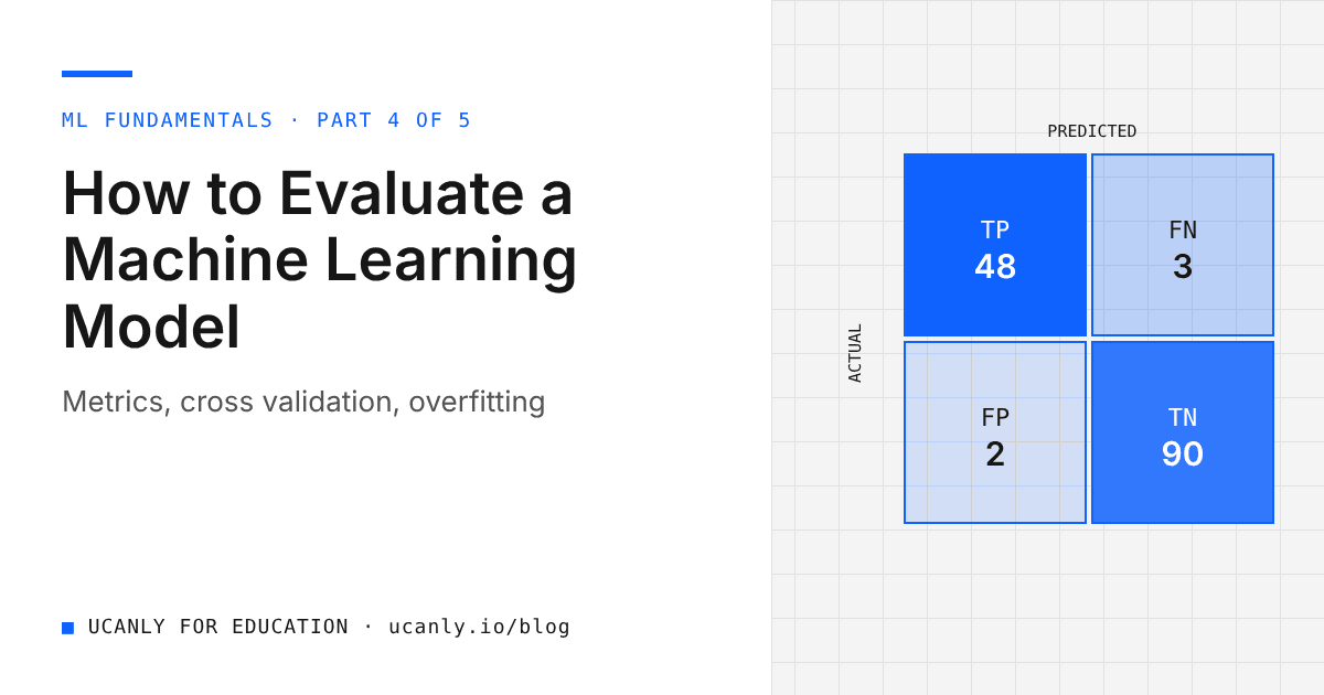
The confusion matrix is a table of counts: rows are actual classes, columns are predicted classes. For a binary problem, the four cells are:
- True Positive (TP): actually positive, predicted positive
- True Negative (TN): actually negative, predicted negative
- False Positive (FP): actually negative, predicted positive (a false alarm)
- False Negative (FN): actually positive, predicted negative (a miss)
In my run, the model made only a couple of mistakes on 114 test samples, with accuracy of roughly 0.98. One detail trips up many students: in load_breast_cancer, label 0 means malignant and 1 means benign. Always check your positive class with target_names before interpreting any metric.
The accuracy trap
Accuracy is correct predictions divided by total predictions. It fails badly when one class is rare, as in fraud detection, disease screening, or predicting which students might drop out of a course. Here is a lazy "model" that always predicts the majority class:
import numpy as np
from sklearn.metrics import accuracy_score, recall_score

# 1000 students, only 20 are actually "at risk" (label 1)
y_true = np.array([1] * 20 + [0] * 980)
y_lazy = np.zeros(1000, dtype=int)   # a model that always predicts 0

print("Accuracy:", accuracy_score(y_true, y_lazy))
print("Recall:", recall_score(y_true, y_lazy))
This prints an accuracy of 0.98 and a recall of 0.0. The model looks excellent and never identifies a single at risk student. This is the most common mistake in student projects built on skewed Kaggle datasets.
Key takeaway: Before reporting accuracy, look at the class distribution with
pd.Series(y).value_counts(). If one class dominates, accuracy alone is not an acceptable headline metric.
Precision, Recall, F1 and ROC AUC
These metrics tell you what kind of mistakes the model makes.
Precision
Precision = TP / (TP + FP). Of everything flagged positive, how much was actually positive? It matters when false alarms are expensive, like a spam filter that must not bury genuine internship offers.
Recall
Recall = TP / (TP + FN). Of all actual positives, how many did the model catch? It matters when misses are expensive, like cancer screening, where missing a malignant case is far worse than an extra test.
F1 Score
F1 is the harmonic mean of precision and recall. It is high only when both are high, making it a good single number for imbalanced problems. Lowering the decision threshold usually raises recall and lowers precision.
classification_report gives all three per class, and the code also computes ROC AUC:
from sklearn.metrics import classification_report, roc_auc_score

print(classification_report(y_test, y_pred, target_names=["malignant", "benign"]))

y_proba = model.predict_proba(X_test)[:, 1]
print("ROC AUC:", round(roc_auc_score(y_test, y_proba), 3))
In my run, both classes showed precision and recall around 0.98 to 0.99. The macro avg row averages classes equally, which is usually the more honest summary on imbalanced data.
ROC AUC
Precision and recall depend on one threshold, usually 0.5. The ROC curve plots true positive rate against false positive rate across all thresholds, and ROC AUC is the area under it.
- An AUC of 0.5 means the model ranks positives no better than random guessing.
- An AUC close to 1.0 means the model almost always ranks a random positive above a random negative.
roc_auc_score needs probabilities, not hard labels, hence predict_proba. The AUC here was roughly 0.99, expected on such a clean dataset. On heavily imbalanced data, also check the precision recall curve, since ROC AUC can look optimistic.
Regression Metrics: MAE, RMSE and R Squared
When the target is a number, such as a house price, you need different metrics.
import numpy as np
from sklearn.datasets import make_regression
from sklearn.linear_model import LinearRegression
from sklearn.metrics import mean_absolute_error, mean_squared_error, r2_score

X_r, y_r = make_regression(n_samples=1000, n_features=8, noise=20, random_state=42)
Xr_train, Xr_test, yr_train, yr_test = train_test_split(
    X_r, y_r, test_size=0.2, random_state=42
)

reg = LinearRegression().fit(Xr_train, yr_train)
yr_pred = reg.predict(Xr_test)

print("MAE :", round(mean_absolute_error(yr_test, yr_pred), 2))
print("RMSE:", round(np.sqrt(mean_squared_error(yr_test, yr_pred)), 2))
print("R2  :", round(r2_score(yr_test, yr_pred), 3))
- MAE: average error size, in target units. Easy to explain.
- RMSE: also in target units, but punishes large mistakes more. If RMSE is much larger than MAE, a few predictions are badly off.
- R squared: share of variance explained. 1.0 is perfect, 0 means no better than predicting the mean, and it can be negative.
Since make_regression is linear by construction, R squared is very high here (roughly 0.98). Real data like California housing gives more modest numbers, which is normal. Always compare against a baseline such as DummyRegressor.
Overfitting, Underfitting and the Bias Variance Tradeoff
Underfitting means the model is too simple: both training and test scores are low. Overfitting means it memorises training noise: training score is very high, test score noticeably lower. Vary the depth of a decision tree to see both:
from sklearn.tree import DecisionTreeClassifier

for depth in [1, 3, 5, None]:
    tree = DecisionTreeClassifier(max_depth=depth, random_state=42)
    tree.fit(X_train, y_train)
    print(f"max_depth={depth}: train={tree.score(X_train, y_train):.3f}, "
          f"test={tree.score(X_test, y_test):.3f}")
In my run, a depth 1 tree scored around 0.92 on both sets. An unrestricted tree hit 1.0 on training data but roughly 0.91 on test data, textbook overfitting. A moderate depth gave the best test score.
This is the bias variance tradeoff in action:
- High bias (underfitting): the model makes strong simplifying assumptions and misses real patterns.
- High variance (overfitting): the model is so flexible that small changes in training data change its predictions a lot.
To reduce overfitting: more data, simpler models, regularisation (C in LogisticRegression), limited tree depth, or ensembles like RandomForestClassifier. To reduce underfitting: better features or a more expressive model.
Key takeaway: Always print both training and validation scores. The gap between them tells you more than either number alone.
Cross Validation and Hyperparameter Tuning
k fold cross validation
A single split can be lucky or unlucky. k fold cross validation splits training data into k parts, trains on k minus 1, validates on the rest, and repeats k times.
from sklearn.model_selection import cross_val_score, StratifiedKFold

cv = StratifiedKFold(n_splits=5, shuffle=True, random_state=42)
scores = cross_val_score(model, X_train, y_train, cv=cv, scoring="f1")
print("F1 per fold:", scores.round(3))
print("Mean F1:", round(scores.mean(), 3), "+/-", round(scores.std(), 3))
In my run, all five F1 scores were close to 0.98 with a small spread, meaning the model is stable. A large spread hints at too little data or overfitting. Run cross validation on the training set only, and use StratifiedKFold for classification.
Tuning with GridSearchCV
Hyperparameters are settings chosen before training, like tree depth. GridSearchCV tries every combination, scores each with cross validation, and keeps the best.
from sklearn.ensemble import RandomForestClassifier
from sklearn.model_selection import GridSearchCV
from sklearn.metrics import make_scorer, recall_score

# In this dataset 0 = malignant, so we ask for recall on class 0
malignant_recall = make_scorer(recall_score, pos_label=0)

param_grid = {
    "n_estimators": [100, 300],
    "max_depth": [None, 5, 10],
    "min_samples_leaf": [1, 3],
}

grid = GridSearchCV(
    RandomForestClassifier(random_state=42),
    param_grid,
    cv=5,
    scoring=malignant_recall,
    n_jobs=-1,
)
grid.fit(X_train, y_train)

print("Best params:", grid.best_params_)
print("Best CV recall (malignant):", round(grid.best_score_, 3))
print("Test recall (malignant):", round(grid.score(X_test, y_test), 3))
Missing a malignant case is the costly error, so we optimise recall on class 0 instead of accuracy. In my run, the best configuration reached a cross validated malignant recall of roughly 0.94, with a similar test value. Be ready to justify your scoring choice in an interview. Keep grids small: fits multiply quickly, so try RandomizedSearchCV for larger searches.
Common Interview Questions on Model Evaluation
These come up regularly in ML internship interviews:
- Why can accuracy be misleading? Give an example.
- When would you prefer precision over recall, and vice versa?
- What does an ROC AUC of 0.5 mean?
- What is the difference between MAE and RMSE, and when would you use each?
- Why do we use cross validation instead of a single validation split?
- How do you detect overfitting, and how do you fix it?
- Explain the bias variance tradeoff in simple words.
- What is data leakage, and how does a
Pipelinehelp prevent it?
Practise answering out loud. Concrete examples, like the lazy model with 98 percent accuracy and zero recall, beat textbook definitions.
What to Do Next
Run every block above in a fresh Colab notebook. Then audit a project you have already built: check class balance, choose metrics that fit the problem, add cross validation, and compare training and test scores. Add a short "Evaluation" section to your README explaining your metric choice. It often impresses reviewers more than the model itself.
For a structured path through ML fundamentals, explore our courses. Then run your resume through the AI resume review so your evaluation work is described clearly, and keep an eye on the jobs board for data and ML internships where you can put these skills to use.