Most machine learning interviews for freshers do not test exotic deep learning. They test whether you truly understand a handful of core algorithms: what each one assumes, when it breaks, and how to use it correctly in code. If you can explain linear regression, logistic regression, k nearest neighbours, decision trees, random forests, support vector machines and k means clustering in plain language, and back that up with clean scikit-learn code, you are ahead of most candidates in a campus placement round.
This guide gives you the intuition for each algorithm, a short runnable example you can paste into Google Colab or a Kaggle notebook, and the interview questions that usually follow. Every dataset used here ships with scikit-learn, so nothing needs to be downloaded.
Before the individual models, fix one mental framework. For every algorithm, ask four questions:
- What does it learn? A line, a set of rules, a boundary, or nothing at all (it just stores the data).
- What does it assume? Linear relationships, scaled features, independent samples.
- How does it fail? Underfitting, overfitting, sensitivity to outliers or to feature scale.
- How do I tune it? The one or two hyperparameters that matter most.
Interviewers rarely ask you to derive formulas. They ask these four questions in different words. Keep them in mind as you read.
Linear and Logistic Regression
Linear regression
Linear regression predicts a number by fitting a weighted sum of the input features. Think of predicting a student's final semester score from attendance, internal marks and hours of study: each feature gets a weight, and the model picks the weights that minimise the squared error between predictions and actual values.
import pandas as pd
from sklearn.datasets import load_diabetes
from sklearn.model_selection import train_test_split
from sklearn.linear_model import LinearRegression
from sklearn.metrics import mean_absolute_error, r2_score

X, y = load_diabetes(return_X_y=True, as_frame=True)
X_train, X_test, y_train, y_test = train_test_split(
    X, y, test_size=0.2, random_state=42
)

model = LinearRegression()
model.fit(X_train, y_train)
pred = model.predict(X_test)

print("MAE:", round(mean_absolute_error(y_test, pred), 2))
print("R2 :", round(r2_score(y_test, pred), 3))
# Each coefficient tells you how the target moves when that feature moves
print(pd.Series(model.coef_, index=X.columns).round(1))
On this split you should see an R squared of roughly 0.45, which is honest: the diabetes dataset is noisy and a straight line explains only part of it. The coefficients are what make linear regression valuable. They tell you the direction and size of each feature's effect, which is why it remains the first model to try on any regression problem.
Watch out for: outliers pulling the line, strongly correlated features (multicollinearity) making coefficients unstable, and relationships that are clearly curved. Ridge and Lasso add a penalty on large weights to control the first two problems.
Logistic regression
Despite the name, logistic regression is a classifier. It computes the same weighted sum, then squashes it through the sigmoid function into a probability between 0 and 1. A threshold, usually 0.5, turns the probability into a class.
from sklearn.datasets import load_breast_cancer
from sklearn.model_selection import train_test_split
from sklearn.pipeline import Pipeline
from sklearn.preprocessing import StandardScaler
from sklearn.linear_model import LogisticRegression
from sklearn.metrics import classification_report, confusion_matrix, roc_auc_score

X, y = load_breast_cancer(return_X_y=True)
X_train, X_test, y_train, y_test = train_test_split(
    X, y, test_size=0.2, stratify=y, random_state=42
)

clf = Pipeline([
    ("scale", StandardScaler()),
    ("model", LogisticRegression(max_iter=1000)),
])
clf.fit(X_train, y_train)

pred = clf.predict(X_test)
proba = clf.predict_proba(X_test)[:, 1]
print(confusion_matrix(y_test, pred))
print(classification_report(y_test, pred))
print("ROC AUC:", round(roc_auc_score(y_test, proba), 3))
With scaling inside a Pipeline, this model reaches roughly 98 percent accuracy and a ROC AUC near 0.99 on the test split. Putting the scaler in the pipeline matters: it is fitted only on training data, so no information leaks from the test set.
Key takeaway: always start a classification project with logistic regression. It is fast, interpretable and gives calibrated probabilities. If a complex model cannot clearly beat it, ship the simple one.
K Nearest Neighbours
KNN learns nothing during training. It simply stores the data. To classify a new point, it finds the k closest training points and takes a majority vote. It is the algorithmic version of "you are the average of the people around you".
Because it relies on distance, feature scaling is mandatory. If one column is salary in rupees and another is CGPA on a 10 point scale, the salary column will dominate every distance calculation.
from sklearn.datasets import load_iris
from sklearn.model_selection import cross_val_score
from sklearn.pipeline import Pipeline
from sklearn.preprocessing import StandardScaler
from sklearn.neighbors import KNeighborsClassifier

X, y = load_iris(return_X_y=True)

for k in [1, 3, 5, 11, 21]:
    knn = Pipeline([
        ("scale", StandardScaler()),
        ("model", KNeighborsClassifier(n_neighbors=k)),
    ])
    scores = cross_val_score(knn, X, y, cv=5)
    print(f"k={k:>2}  mean accuracy={scores.mean():.3f}")
In this run, very small k (k=1) memorises noise, and very large k blurs class boundaries. A middle value such as k=5 scored best, around 96 percent. That is the bias and variance tradeoff in one loop.
Watch out for: slow predictions on large datasets (every prediction scans the training data) and poor performance with many irrelevant features, often called the curse of dimensionality.
Decision Trees and Random Forests
Decision trees
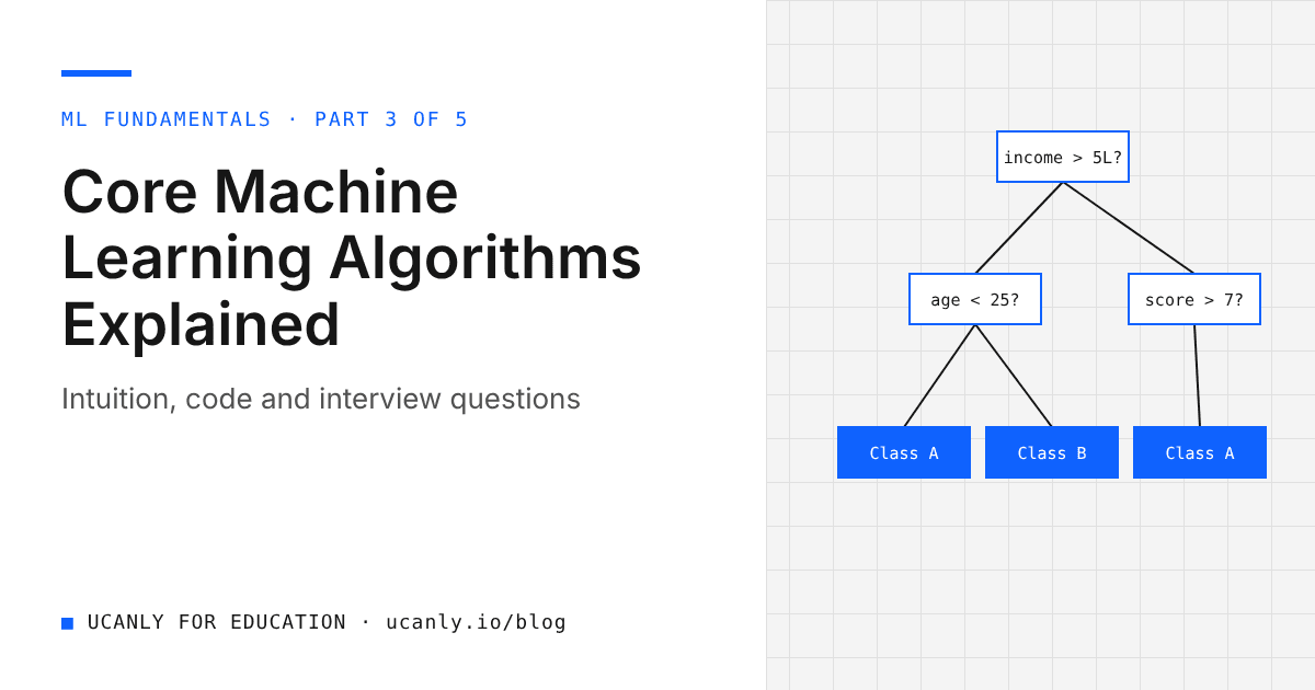
A decision tree asks a sequence of yes or no questions about the features, choosing at each step the split that best separates the classes (measured by Gini impurity or entropy). It is exactly how a placement cell might shortlist: "CGPA above 7? Has an internship? Cleared the aptitude test?"
from sklearn.datasets import load_breast_cancer
from sklearn.model_selection import train_test_split
from sklearn.tree import DecisionTreeClassifier, export_text

data = load_breast_cancer()
X_train, X_test, y_train, y_test = train_test_split(
    data.data, data.target, test_size=0.2, stratify=data.target, random_state=42
)

for depth in [None, 3]:
    tree = DecisionTreeClassifier(max_depth=depth, random_state=42)
    tree.fit(X_train, y_train)
    print(f"max_depth={depth}: train={tree.score(X_train, y_train):.3f} "
          f"test={tree.score(X_test, y_test):.3f}")

# Print the rules of the shallow tree in plain text
print(export_text(tree, feature_names=list(data.feature_names)))
The unrestricted tree scores a perfect 1.0 on training data but drops to about 0.91 on the test set. Limiting depth to 3 lowers training accuracy yet improves test accuracy to roughly 0.94. That gap is overfitting, and it is the single most common decision tree interview topic. export_text prints the learned rules, which is why trees are loved for explainability.
Random forests
A random forest trains hundreds of trees, each on a random bootstrap sample of rows and a random subset of features at each split, then averages their votes. Individual trees overfit in different directions, so averaging cancels much of the noise. This idea is called bagging.
import pandas as pd
from sklearn.datasets import load_breast_cancer
from sklearn.model_selection import train_test_split
from sklearn.ensemble import RandomForestClassifier

data = load_breast_cancer()
X_train, X_test, y_train, y_test = train_test_split(
    data.data, data.target, test_size=0.2, stratify=data.target, random_state=42
)

forest = RandomForestClassifier(n_estimators=300, random_state=42, n_jobs=-1)
forest.fit(X_train, y_train)
print("Test accuracy:", round(forest.score(X_test, y_test), 3))

importance = pd.Series(forest.feature_importances_, index=data.feature_names)
print(importance.sort_values(ascending=False).head(5))
The forest reaches around 95 percent test accuracy here with almost no tuning, and feature_importances_ shows which measurements drove the predictions. For tabular data in college projects and hackathons, a random forest is a strong, low effort baseline. Gradient boosting libraries are the natural next step once you are comfortable with forests.
Support Vector Machines, Briefly
An SVM looks for the boundary that separates classes with the widest possible margin. Only the points closest to the boundary, the support vectors, decide where it sits. With the RBF kernel, SVMs can draw curved boundaries without you engineering new features.
from sklearn.datasets import load_breast_cancer
from sklearn.model_selection import cross_val_score
from sklearn.pipeline import Pipeline
from sklearn.preprocessing import StandardScaler
from sklearn.svm import SVC

X, y = load_breast_cancer(return_X_y=True)
svm = Pipeline([
    ("scale", StandardScaler()),
    ("model", SVC(kernel="rbf", C=1.0, gamma="scale")),
])
print("CV accuracy:", round(cross_val_score(svm, X, y, cv=5).mean(), 3))
This gives a cross validated accuracy of roughly 97 percent. The two knobs to know are C (how much to penalise misclassified points; higher C means a tighter fit) and gamma (how far the influence of a single point reaches). SVMs need scaled features and become slow on very large datasets, which is why they appear less often in modern production pipelines but still feature regularly in interviews.
K Means Clustering
Everything so far was supervised: we had labels. K means is unsupervised. You choose k, the algorithm places k centroids, assigns each point to its nearest centroid, moves each centroid to the mean of its points, and repeats until nothing changes. Typical uses include grouping students by learning behaviour on an ed tech platform or segmenting customers for a marketing internship project.
from sklearn.datasets import load_iris
from sklearn.preprocessing import StandardScaler
from sklearn.cluster import KMeans
from sklearn.metrics import silhouette_score

X, _ = load_iris(return_X_y=True)   # we ignore the labels on purpose
X_scaled = StandardScaler().fit_transform(X)

for k in range(2, 7):
    km = KMeans(n_clusters=k, n_init=10, random_state=42)
    labels = km.fit_predict(X_scaled)
    print(f"k={k}  inertia={km.inertia_:.1f}  silhouette={silhouette_score(X_scaled, labels):.3f}")
Here is a useful lesson. Iris has three species, yet the silhouette score is highest at k=2, because two of the species overlap heavily in feature space. Inertia always falls as k grows, so you look for an "elbow" rather than the minimum. Clustering metrics guide you; they do not hand you the truth. Domain knowledge decides the final k.
Watch out for: unscaled features, clusters that are not roughly spherical, and sensitivity to the random starting centroids (which n_init addresses by running several initialisations).
When to Use Which: A Comparison
Compare models fairly with the same cross validation folds and the same metric:
from sklearn.datasets import load_breast_cancer
from sklearn.model_selection import cross_val_score, StratifiedKFold
from sklearn.pipeline import make_pipeline
from sklearn.preprocessing import StandardScaler
from sklearn.linear_model import LogisticRegression
from sklearn.neighbors import KNeighborsClassifier
from sklearn.tree import DecisionTreeClassifier
from sklearn.ensemble import RandomForestClassifier
from sklearn.svm import SVC

X, y = load_breast_cancer(return_X_y=True)
cv = StratifiedKFold(n_splits=5, shuffle=True, random_state=42)

models = {
    "Logistic Regression": make_pipeline(StandardScaler(), LogisticRegression(max_iter=1000)),
    "KNN (k=5)": make_pipeline(StandardScaler(), KNeighborsClassifier()),
    "Decision Tree": DecisionTreeClassifier(max_depth=4, random_state=42),
    "Random Forest": RandomForestClassifier(n_estimators=300, random_state=42),
    "SVM (RBF)": make_pipeline(StandardScaler(), SVC()),
}

for name, model in models.items():
    scores = cross_val_score(model, X, y, cv=cv, scoring="roc_auc")
    print(f"{name:<20} ROC AUC {scores.mean():.3f} +/- {scores.std():.3f}")
On this dataset logistic regression and the RBF SVM land near 0.995 ROC AUC, the random forest close behind, and a single shallow tree clearly lowest with the largest spread. Results will differ on other data, which is the point: always test, never assume.
Use this list as a quick decision guide:
- Linear regression: predicting a continuous number when you want interpretable coefficients. Always your regression baseline.
- Logistic regression: binary or multiclass classification baseline; when you need probabilities and explainability.
- KNN: small, low dimensional datasets; quick prototypes; recommendation style "find similar items" problems.
- Decision tree: when stakeholders need readable rules; rarely the best scorer on its own.
- Random forest: default strong choice for tabular data with mixed feature types and little tuning time.
- SVM: small to medium datasets with complex boundaries, such as text classification with many features.
- K means: no labels, and you want to discover natural groups in the data.
Key takeaway: in an interview, the best answer to "which algorithm would you use?" is "I would start with a simple baseline, then compare a few candidates using cross validation on the metric that matches the business goal."
Typical Interview Questions
Prepare short, spoken answers to these. Practise saying them aloud.
Linear regression
- What assumptions does linear regression make, and what happens when they are violated?
- What is the difference between Ridge (L2) and Lasso (L1) regularisation? Why can Lasso set coefficients to exactly zero?
- Why is R squared alone not enough to judge a model?
Logistic regression
- Why is it called regression if it is used for classification?
- Why do we use log loss instead of mean squared error?
- How would you change the decision threshold for a fraud detection problem where missing fraud is very costly?
KNN
- Why must features be scaled for KNN?
- What happens when k is 1? When k equals the number of training samples?
Decision trees and random forests
- How does a tree choose a split? Explain Gini impurity in simple words.
- How does a random forest reduce overfitting compared to one tree?
- What is the difference between bagging and boosting?
SVM
- What are support vectors, and what is the kernel trick?
- What do the
Candgammaparameters control?
K means
- How do you choose k? Explain the elbow method and silhouette score.
- Why can k means give different results on different runs?
If you want structured practice beyond this list, our courses walk through each algorithm with guided notebooks and assignments.
What to Do Next
Do not just read this. Open a Colab notebook today and run every code block above, then change one thing each time: a different max_depth, a different k, removing the scaler. Watching the scores move builds the intuition interviewers look for.
Next, pick one dataset relevant to you, such as placement outcomes, hostel mess feedback or local rainfall, and apply the comparison loop end to end. Write a short README explaining which model you chose and why. That single, well documented project is worth more than ten copied notebooks.
Finally, add the project to your resume with the metric you optimised and the reason behind your model choice. Run it through our AI resume review to sharpen the wording, and when you feel ready, start applying through the jobs board. Master these seven algorithms properly and every advanced topic you learn later will make far more sense.