Your First End to End Machine Learning Project on Google Colab: From Problem Definition to GitHub

Most students learn machine learning in fragments. One video on logistic regression, one notebook on random forests, a Kaggle kernel copied without understanding. Then a placement interviewer asks, "Walk me through a project you built from start to finish," and the fragments do not add up to an answer.

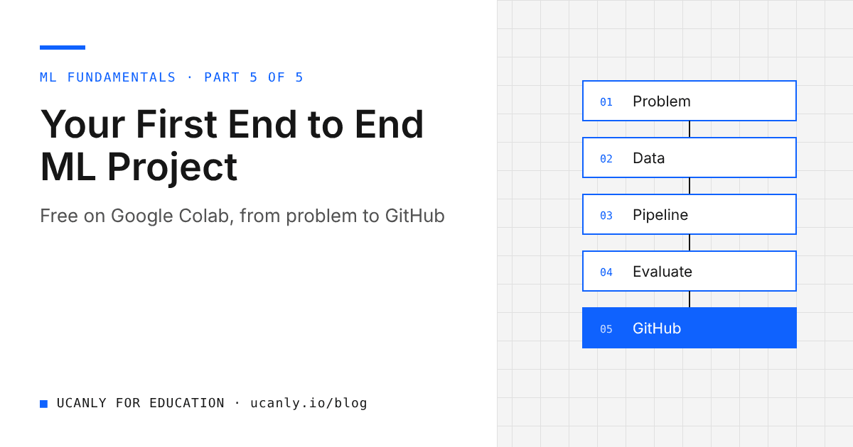
This guide fixes that. You will build one complete, honest machine learning project on Google Colab, entirely free, using a dataset that ships with scikit-learn. You will define the problem, explore the data, build a Pipeline, compare two models with cross validation, evaluate once on a held out test set, save the model, write a prediction function, and publish it on GitHub. At the end you get a 30 day roadmap and a script for talking about the project in interviews.

Part 1: Problem Definition and Data

Define the Problem Before You Touch Code

Open a new notebook at colab.research.google.com and write a Markdown cell at the top answering four questions:

• What are we predicting? Whether a breast tumour is malignant or benign, based on measurements computed from a digitised image of a cell sample.
• What type of problem is it? Binary classification.
• Who would use it and why? A screening assistant that flags suspicious cases for a doctor. It supports a decision, it does not replace one.
• What does a mistake cost? Calling a malignant tumour benign (a false negative for cancer) is far worse than the reverse. So recall on the malignant class matters more than raw accuracy.

That last point is the one interviewers love. It shows you think about consequences, not just scores.

Key takeaway: write the problem statement and the cost of errors first. It decides which metric you optimise.

Load and Explore the Data

The Wisconsin breast cancer dataset loads instantly, with no downloads or API keys.

import pandas as pd
from sklearn.datasets import load_breast_cancer

data = load_breast_cancer(as_frame=True)
df = data.frame
print(df.shape)
print(data.target_names)
print(df["target"].value_counts())

You should see 569 rows and 31 columns: 30 numeric features plus target. Pay close attention to the label encoding: 0 means malignant and 1 means benign. Many beginners assume 1 means "has cancer" and then misread every metric. Note it in your README.

The classes are imbalanced, roughly 60 percent benign and 40 percent malignant, which is why we will stratify the split.

Now explore:

print(df.isnull().sum().sum())
print(df[["mean radius", "mean texture", "mean area"]].describe())
print(df.groupby("target")[["mean radius", "mean concave points"]].mean())

There are no missing values, and the features sit on very different scales (area is in the hundreds, smoothness is a small fraction). The group means show malignant samples tend to have a larger radius and more concave points. Write two or three such observations in Markdown cells. Exploration you never write down is exploration the reader assumes you skipped.

Part 2: Pipeline and Model Comparison

Split First, Then Build a Pipeline

Split before any preprocessing so the test set stays genuinely unseen.

from sklearn.model_selection import train_test_split

X = df.drop(columns="target")
y = df["target"]

X_train, X_test, y_train, y_test = train_test_split(
    X, y, test_size=0.2, stratify=y, random_state=42
)
print(X_train.shape, X_test.shape)

Now wrap preprocessing and the model inside a Pipeline. This guarantees the scaler learns its mean and standard deviation only from training folds, which prevents data leakage during cross validation.

from sklearn.pipeline import Pipeline
from sklearn.impute import SimpleImputer
from sklearn.preprocessing import StandardScaler
from sklearn.linear_model import LogisticRegression
from sklearn.ensemble import RandomForestClassifier

log_reg = Pipeline([
    ("imputer", SimpleImputer(strategy="median")),
    ("scaler", StandardScaler()),
    ("model", LogisticRegression(max_iter=1000)),
])

forest = Pipeline([
    ("imputer", SimpleImputer(strategy="median")),
    ("model", RandomForestClassifier(n_estimators=200, random_state=42)),
])

The imputer does nothing today because there are no missing values, but it makes the pipeline robust if a future input row arrives with a blank field. Random forests do not need scaling, so that pipeline skips it.

Compare Two Models With Cross Validation

Never pick a model based on one lucky split. Use five fold cross validation on the training set only.

from sklearn.model_selection import cross_val_score

for name, pipe in [("Logistic Regression", log_reg), ("Random Forest", forest)]:
    scores = cross_val_score(pipe, X_train, y_train, cv=5, scoring="roc_auc")
    print(f"{name}: mean ROC AUC {scores.mean():.3f} (std {scores.std():.3f})")

In our run both models scored very high, with logistic regression around 0.99 ROC AUC and the random forest only slightly behind. When two models are this close, prefer the simpler one: logistic regression is faster, easier to explain, and its coefficients tell you which features push a prediction toward malignant. That reasoning is worth more in an interview than the decimal points.

Key takeaway: cross validation is for choosing a model. The test set is for reporting the final result, once.

Part 3: Evaluate, Save and Predict

Evaluate Once on the Held Out Test Set

from sklearn.metrics import classification_report, confusion_matrix, roc_auc_score

best = log_reg
best.fit(X_train, y_train)

y_pred = best.predict(X_test)
y_proba = best.predict_proba(X_test)[:, 1]

print(confusion_matrix(y_test, y_pred))
print(classification_report(y_test, y_pred, target_names=data.target_names))
print("Test ROC AUC:", round(roc_auc_score(y_test, y_proba), 3))

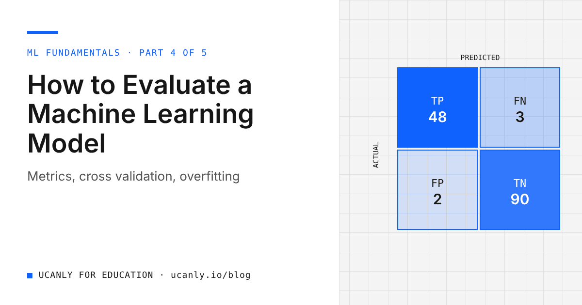
In our run, accuracy on the 114 test samples was roughly 98 percent, with only a couple of misclassifications in the confusion matrix. Your numbers may differ slightly. Read the matrix row by row: the first row is actual malignant cases, so any count in its second column is a cancer case the model called benign. That is the number your problem statement told you to watch.

Be honest in your README: this is a small, clean, well studied dataset. High scores here do not mean the model is ready for a hospital. Saying so signals maturity.

Save the Model and Write a Prediction Function

import joblib

joblib.dump(best, "breast_cancer_model.joblib")

def predict_tumour(features: dict, model_path="breast_cancer_model.joblib"):
    model = joblib.load(model_path)
    row = pd.DataFrame([features], columns=X.columns)
    proba_benign = model.predict_proba(row)[0, 1]
    label = "benign" if proba_benign >= 0.5 else "malignant"
    return {"prediction": label, "probability_benign": round(float(proba_benign), 3)}

sample = X_test.iloc[0].to_dict()
print(predict_tumour(sample))

Because you saved the whole Pipeline, the scaler travels with the model. Anyone who loads the file gets identical preprocessing automatically. In Colab, download the .joblib file from the Files panel on the left so you can commit it to GitHub. Note that joblib files should only be loaded from sources you trust, and they are tied to the library versions used to create them, so record your scikit-learn version.

Part 4: Publish on GitHub With a Good README

Download your notebook with File, Download, Download .ipynb. Create a public repository and organise it like this:

breast-cancer-classifier/
  README.md
  notebook.ipynb
  predict.py
  breast_cancer_model.joblib
  requirements.txt

Put predict_tumour in predict.py, and list pandas, scikit-learn and joblib with versions in requirements.txt. Your README should contain:

1. Problem statement in two lines, including why false negatives matter.
2. Dataset with source, size, and the label encoding (0 malignant, 1 benign).
3. Approach: Pipeline, two models, five fold cross validation, held out test set.
4. Results as a small table of cross validation and test scores, written as approximate.
5. How to run, with the exact commands and a usage example of the prediction function.
6. Limitations and next steps, such as threshold tuning to raise malignant recall.

A recruiter spends very little time on a repository. A clear README is what makes those seconds count. Once it is live, add the link to your resume and run it through our AI resume review to check that the project bullet reads well.

A 30 Day ML Fundamentals Roadmap

Spend about one to two hours a day. Consistency beats weekend marathons.

Week 1: Python and Data Handling

• Days 1 to 3: pandas basics: selecting, filtering, groupby, merging.
• Days 4 to 5: numpy arrays and broadcasting.
• Days 6 to 7: plotting distributions and correlations with matplotlib or seaborn.

Week 2: Core Supervised Learning

• Days 8 to 10: linear and logistic regression, what a loss function is, overfitting.
• Days 11 to 12: decision trees and random forests.
• Days 13 to 14: train test split, cross validation, and data leakage.

Week 3: Evaluation and Pipelines

• Days 15 to 17: confusion matrix, precision, recall, F1, ROC AUC, and when each matters.
• Days 18 to 19: Pipeline and ColumnTransformer on a mixed dataset such as seaborn titanic.
• Days 20 to 21: hyperparameter tuning with GridSearchCV.

Week 4: Build and Ship

• Days 22 to 26: rebuild this project from memory, then repeat the workflow on a regression problem using fetch_california_housing.
• Days 27 to 28: polish both READMEs.
• Days 29 to 30: rehearse your interview explanation out loud and record yourself.

If you want this structured with checkpoints, our courses follow a similar progression.

How to Talk About This Project in Placement Interviews

Use a simple structure: problem, data, approach, result, learning. A strong two minute answer sounds like this:

"I built a binary classifier to flag malignant breast tumours from 30 cell measurements. Since missing a malignant case is costly, I focused on malignant recall, not just accuracy. I wrapped scaling and the model in a scikit learn Pipeline to avoid leakage, compared logistic regression and a random forest with five fold cross validation, and chose logistic regression because it matched the forest closely while being simpler to explain. On a held out test set it reached roughly 98 percent accuracy. I saved the pipeline with joblib and published it with a prediction function and README."

Then prepare for follow up questions:

• Why did you scale features for logistic regression but not the random forest?
• What is data leakage, and how did your Pipeline prevent it?
• Why is accuracy misleading on imbalanced data?
• What is the difference between precision and recall? Which mattered more here?
• How would you reduce false negatives? (Lower the decision threshold and accept more false positives.)
• What does ROC AUC measure?
• Why use cross validation instead of a single validation split?

If you cannot answer one of these confidently, that is your next study topic. Interviewers rarely expect a novel model from a fresher. They expect you to understand every line you wrote.

What to Do Next

Open Colab today and rebuild this project yourself instead of just reading it. Push it to GitHub with a proper README within the week. Then start the 30 day roadmap, and add a second project on a regression dataset so you can show range. When your portfolio has two clean, explainable projects, start applying through our jobs board and keep reading the blog for the next topics in this series.

One project you understand completely is worth more than ten you copied.